
2021年9月4日公開 著者:Edvin Hopkins
Pythonには、数値計算やデータ可視化のための優れたパッケージがあります。例えば、numpy、scipy、matplotlibなどです。最近注目を集めているもう一つのパッケージとして、Pythonのpandasライブラリがあります。pandasは、大量のデータを保存・処理するための高速で効率的なデータ分析ツールを提供しています。これらのパッケージはすべて、nAG Library for Pythonと簡単に統合できます。
以下は、nAG Library for Pythonとpandasライブラリを使用して、オプション価格のインプライド・ボラティリティを計算する例です。このコードをダウンロードすれば、シカゴ・オプション取引所のウェブサイトからデータを取得し、独自のインプライド・ボラティリティ・サーフェスを計算することができます。nAGライブラリ製品の全機能トライアルを利用できます - 詳細はブログ末尾のリンクをご覧ください。
インプライド・ボラティリティの背景
株式オプションの価格を算出する有名なブラック・ショールズの公式は、6つの変数の関数です:原資産価格、金利、配当率、行使価格、満期までの期間、そしてボラティリティです。特定のオプション契約では、原資産価格、金利、配当率を観察することができます。さらに、オプション契約では行使価格と満期までの期間が指定されています。
したがって、調整する必要がある唯一の変数はボラティリティです。そこで次の問題を考えることができます:どのようなボラティリティ*を用いれば、ブラック・ショールズ方程式の価格が市場価格と等しくなるか。
F(ボラティリティ*) = Market Option Price
このボラティリティ*が、市場で観察されるインプライド・ボラティリティと呼ばれます。nAGルーチンのopt_imp_volを使用して、入力データの配列に対するインプライド・ボラティリティを計算することができます。
このルーチンはMark 27.1で導入され、ユーザーは2つのアルゴリズムから選択できます。1つ目はJäckel (2015)の方法で、3次のハウスホルダー法を使用して、極端な入力を除くほぼすべての場合で機械精度に近い精度を達成します。この方法は、短いベクトルの入力データに対して高速です。
2つ目のアルゴリズムは、Glau et al. (2018)の方法をベースにしており、nAGとロンドン大学クイーン・メアリー校のKathrin Glau博士およびLinus Wunderlich博士との非常に生産的な共同研究によって開発された追加のパフォーマンス向上機能が含まれています。この方法はチェビシェフ補間を使用し、長いベクトルの入力データに対して設計されており、SIMDベクトル命令を活用してパフォーマンスを向上させることができます。機械精度の精度が必要ない用途では、このアルゴリズムに単精度(約7桁の小数点)程度の精度を目指すよう指示することもでき、さらなるパフォーマンス向上が得られます。
インプライド・ボラティリティを計算した後、dim2_cheb_linesを使用してボラティリティ・サーフェスに最小二乗チェビシェフフィットを行い、dim2_cheb_evalを使用して中間点でサーフェスを評価することができます。
必要なパッケージ
このスクリプトは以下のパッケージで動作確認されています:
- Python 3.8
- numpy 1.16.4
- pandas 0.24.2
- matplotlib 3.1.0
- nAG Library for Python
コードの説明
以下は、インプライド・ボラティリティを計算し、ボラティリティ曲線とサーフェスをプロットするPythonスクリプトの完全なコードです。
#!/usr/bin/env python3

"""
Example for Implied Volatility using the nAG Library for Python
Finds implied volatilities of the Black Scholes equation using specfun.opt_imp_vol
Data needs to be downloaded from:
http://www.cboe.com/delayedquote/QuoteTableDownload.aspx
Make sure to download data during CBOE Trading Hours.

Updated for nAG Library for Python Mark 27.1
"""

# pylint: disable=invalid-name,too-many-branches,too-many-locals,too-many-statements

try:
    import sys
    import pandas
    import numpy as np
    import matplotlib.pylab as plt
    import warnings
    from naginterfaces.library import specfun, fit
    from naginterfaces.base import utils
    from matplotlib import cm

except ImportError as e:
    print(
        "Could not import the following module. "
        "Do you have a working installation of the nAG Library for Python?"
    )
    print(e)
    sys.exit(1)

__author__ = "Edvin Hopkins, John Morrissey and Brian Spector"
__copyright__ = "Copyright 2021, The Numerical Algorithms Group Inc"
__email__ = "support@nag.co.uk"

# Set to hold expiration dates
dates = []

cumulative_month = {'Jan': 31, 'Feb': 57, 'Mar': 90,
                    'Apr': 120, 'May': 151, 'Jun': 181,
                    'Jul': 212, 'Aug': 243, 'Sep': 273,
                    'Oct': 304, 'Nov': 334, 'Dec': 365}

def main(): # pylint: disable=missing-function-docstring

    try:
        if len(sys.argv)>1:
            QuoteData = sys.argv[1]
        else:
            QuoteData = 'QuoteData.dat'

        qd = open(QuoteData, 'r')
        qd_head = []
        qd_head.append(qd.readline())
        qd_head.append(qd.readline())
        qd.close()
    except: # pylint: disable=bare-except
        sys.stderr.write("Usage: implied_volatility.py QuoteData.dat\n")
        sys.stderr.write("Couldn't read QuoteData\n")
        sys.exit(1)

    print("Implied Volatility for %s %s" % (qd_head[0].strip(), qd_head[1]))

    # Parse the header information in QuotaData
    first = qd_head[0].split(',')
    second = qd_head[1].split()
    qd_date = qd_head[1].split(',')[0]

    company = first[0]
    underlyingprice = float(first[1])
    month, day = second[:2]
    today = cumulative_month[month] + int(day) - 30
    current_year = int(second[2])

    def getExpiration(x):
        monthday = x.split()
        adate = monthday[0] + ' ' + monthday[1]
        if adate not in dates:
            dates.append(adate)
        return (int(monthday[0]) - (current_year % 2000)) * 365 + cumulative_month[monthday[1]]

    def getStrike(x):
        monthday = x.split()
        return float(monthday[2])

    data = pandas.io.parsers.read_csv(QuoteData, sep=',', header=2, na_values=' ')

    # Need to fill the NA values in dataframe
    data = data.fillna(0.0)

    # Let's look at data where there was a recent sale
    data = data[(data['Last Sale'] > 0) | (data['Last Sale.1'] > 0)]

    # Get the Options Expiration Date
    exp = data.Calls.apply(getExpiration)
    exp.name = 'Expiration'

    # Get the Strike Prices
    strike = data.Calls.apply(getStrike)
    strike.name = 'Strike'

    data = data.join(exp).join(strike)

    print("Number of data points found: {}\n".format(len(data.index)))

    print('Calculating Implied Vol of Calls...')
    r = np.zeros(len(data.index))
    t = (data.Expiration - today)/365.0
    s0 = np.full(len(data.index),underlyingprice)
    pCall= (data.Bid + data.Ask) / 2

    # A lot of the data is incomplete or extreme so we tell the nAG routine
    # not to worry about warning us about data points it can't work with
    warnings.simplefilter('ignore',utils.NagAlgorithmicWarning)
    sigmaCall = specfun.opt_imp_vol('C',pCall,data.Strike, s0,t,r,mode = 1).sigma
    impvolcall = pandas.Series(sigmaCall,index=data.index, name='impvolCall')

    data = data.join(impvolcall)

    print('Calculating Implied Vol of Puts...')
    pPut= (data['Bid.1'] + data['Ask.1']) / 2
    sigmaPut = specfun.opt_imp_vol('P',pPut,data.Strike, s0,t,r,mode = 1).sigma
    impvolput = pandas.Series(sigmaPut,index=data.index, name='impvolPut')

    data = data.join(impvolput)
    fig = plt.figure(1)
    fig.subplots_adjust(hspace=.4, wspace=.3)

    # Plot the Volatility Curves
    # Encode graph layout: 3 rows, 3 columns, 1 is first graph.
    num = 331
    max_xticks = 4

    for date in dates:
        # add each subplot to the figure
        plot_year, plot_month = date.split()
        plot_date = (int(plot_year) - (current_year % 2000)) * 365 + cumulative_month[plot_month]
        plot_call = data[(data.impvolCall > .01) &
                       (data.Expiration == plot_date) &
                       (data['Last Sale'] > 0)]
        plot_put = data[(data.impvolPut > .01) &
                        (data.Expiration == plot_date) &
                        (data['Last Sale.1'] > 0)]

        myfig = fig.add_subplot(num)
        xloc = plt.MaxNLocator(max_xticks)
        myfig.xaxis.set_major_locator(xloc)
        myfig.set_title('Expiry: %s 20%s' % (plot_month, plot_year))
        myfig.plot(plot_call.Strike, plot_call.impvolCall, 'pr', label='call',markersize=0.5)
        myfig.plot(plot_put.Strike, plot_put.impvolPut, 'p', label='put',markersize=0.5)
        myfig.legend(loc=1, numpoints=1, prop={'size': 10})
        myfig.set_ylim([0,1])
        myfig.set_xlabel('Strike Price')
        myfig.set_ylabel('Implied Volatility')
        num += 1

    plt.suptitle('Implied Volatility for %s Current Price: %s Date: %s' %
                 (company, underlyingprice, qd_date))


    print("\nPlotting Volatility Curves/Surface")

    # The code below will plot the Volatility Surface
    # It uses fit.dim2_cheb_lines to fit with a polynomial and
    # fit.dim2_cheb_eval to evaluate at intermediate points

    m = np.empty(len(dates), dtype=np.int32)
    y = np.empty(len(dates), dtype=np.double)
    xmin = np.empty(len(dates), dtype=np.double)
    xmax = np.empty(len(dates), dtype=np.double)

    data = data.sort_values(by=['Strike']) # Need to sort for nAG Algorithm

    k = 3   # this is the degree of polynomial for x-axis (Strike Price)
    l = 3   # this is the degree of polynomial for y-axis (Expiration Date)

    i = 0

    for date in dates:
        plot_year, plot_month = date.split()
        plot_date = (int(plot_year) - (current_year % 2000)) * 365 + cumulative_month[plot_month]

        call_data = data[(data.Expiration == plot_date) &
                (data.impvolPut > .01) &
                (data.impvolPut < 1) &
                                (data['Last Sale.1'] > 0)]

        exp_sizes = call_data.Expiration.size
        if exp_sizes > 0:
            m[i] = exp_sizes

            if i == 0:
                x = np.array(call_data.Strike)
                call = np.array(call_data.impvolPut)
                xmin[0] = x.min()
                xmax[0] = x.max()
            else:
                x2 = np.array(call_data.Strike)
                x = np.append(x,x2)
                call2 = np.array(call_data.impvolPut)
                call = np.append(call,call2)
                xmin[i] = x2.min()
                xmax[i] = x2.max()
            y[i] = plot_date-today
            i+=1
    nux = np.zeros(1,dtype=np.double)
    nuy = np.zeros(1,dtype=np.double)

    if len(dates) != i:
        print(
            "Error with data: the CBOE may not be open for trading "
            "or one expiration date has null data"
        )
        return 0
    weight = np.ones(call.size, dtype=np.double)

    #Call the nAG Chebyshev fitting function
    output_coef = fit.dim2_cheb_lines(m,k,l,x,y,call,weight,(k + 1) * (l + 1),xmin,xmax,nux,nuy)

    # Now that we have fit the function,
    # we use fit.dim2_cheb_eval to evaluate at different strikes/expirations

    nStrikes = 100 # number of Strikes to evaluate
    spacing = 20 # number of Expirations to evaluate

    for i in range(spacing):
        mfirst = 1
        xmin = data.Strike.min()
        xmax = data.Strike.max()

        x = np.linspace(xmin, xmax, nStrikes)

        ymin = data.Expiration.min() - today
        ymax = data.Expiration.max() - today

        y = (ymin) + i * np.floor((ymax - ymin) / spacing)

        fx=np.empty(nStrikes)

        fx=fit.dim2_cheb_eval(mfirst,k,l,x,xmin,xmax,y,ymin,ymax,output_coef)

        if 'xaxis' in locals():
            xaxis = np.append(xaxis, x)
            temp = np.empty(len(x))
            temp.fill(y)
            yaxis = np.append(yaxis, temp)
            for j in range(len(x)):
                zaxis.append(fx[j])
        else:
            xaxis = x
            yaxis = np.empty(len(x), dtype=np.double)
            yaxis.fill(y)
            zaxis = []
            for j in range(len(x)):
                zaxis.append(fx[j])

    fig = plt.figure(2)
    ax = fig.add_subplot(111, projection='3d')

    # A try-except block for Matplotlib
    try:
        ax.plot_trisurf(xaxis, yaxis, zaxis, cmap=cm.jet)
    except AttributeError:
        print ("Your version of Matplotlib does not support plot_trisurf")
        print ("...plotting wireframe instead")
        ax.plot(xaxis, yaxis, zaxis)

    ax.set_xlabel('Strike Price')
    ax.set_ylabel('Days to Expiration')
    ax.set_zlabel('Implied Volatility for Put Options')
    plt.suptitle('Implied Volatility Surface for %s Current Price: %s Date: %s' %
                 (company, underlyingprice, qd_date))

    plt.show()

if __name__ == "__main__":
    main()
スクリプトの実行
実行手順
- データの準備:
- QuoteData.dat をスクリプトがあるフォルダに配置します。
- スクリプトの実行:
コマンドラインでスクリプトのあるフォルダに移動して、以下のコマンドを実行します:
python implied_volatility.py ./data/QuoteData.dat
出力結果
スクリプトを実行すると、以下のような出力が得られます:
Implied Volatility for AAPL (APPLE INC),546.0255,-4.7445, Dec 19 2013 @ 15:02 ET,Bid,545.97,Ask,546.09,Size,2×1,Vol,8897300,

Number of data points found: 17905

Calculating Implied Vol of Calls...

Calculating Implied Vol of Puts...

Plotting Volatility Curves/Surface
また、2つのグラフが表示されます:
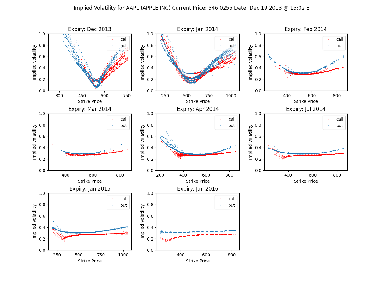
- ボラティリティ曲線:
- 複数のサブプロットで構成され、各サブプロットは異なる満期日のコールオプションとプットオプションのインプライド・ボラティリティを示します。
- ボラティリティ・サーフェス:
- 3Dグラフで、x軸が行使価格、y軸が満期までの日数、z軸がプットオプションのインプライド・ボラティリティを表します。
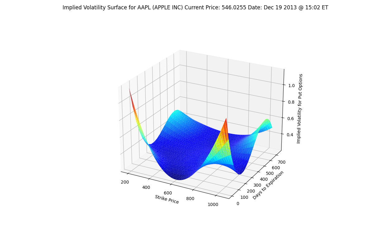
これらのグラフから、オプションの満期日が長くなるにつれてボラティリティのスキュー/スマイルが平坦化する傾向が観察できます。この視覚化により、実際のオプション価格とブラック・ショールズモデルの想定との差異を直感的に理解することができます。
さて、これで準備が整いました。提供されたQuoteDataを使って、独自のボラティリティ・サーフェスをプロットしてみましょう。このスクリプトを実行することで、データ分析や可視化の実践的な例を体験でき、金融工学や数値計算の学習に役立つはずです。
なお、このコードの作成にあたり、John MorrisseyとChris Seymourから貴重な提案をいただきました。ここに感謝の意を表します。
インプライド・ボラティリティの計算におけるnAGライブラリの活用について、さらに詳しく知りたい方は、nAGライブラリのインプライド・ボラティリティのページをご覧ください。