
このページは、nAGライブラリのJupyterノートブックExampleの日本語翻訳版です。オリジナルのノートブックはインタラクティブに操作することができます。
最近相関行列
このノートブックでは、nAG Library for Pythonを使用して最近相関行列を計算することについて見ていきます。
相関行列
\(n\) × \(n\)行列が相関行列であるための条件は以下の通りです:
- 対称行列である
- 対角線上に1が並んでいる
- 固有値が非負である(正半定値)
\[ \Large Ax = \lambda x, \quad x \neq 0\]
\(i\)行\(j\)列の要素は、\(i\)番目と\(j\)番目の変数間の相関を表します。これは例えば株価のプロセスなどが考えられます。
経験的相関行列
経験的相関行列は、データの不整合や欠損のため、しばしば数学的に真の相関行列ではありません。
そのため、入力\(G\)が近似的な相関行列である場合に、真の相関行列を見つける必要があります。
特に、ほとんどの場合、最近傍相関行列を求めます。
相関行列の計算
- ベクトル\(p_i\)は行列\(P\)の\(i\)列目で、\(n\)個ある変数の\(i\)番目の変数の\(m\)個の観測値を保持しています。\(\bar{p}_i\)はサンプル平均です。
\[ \large S_{ij}=\frac{1}{m-1}(p_i - \bar{p}_i )^T(p_j - \bar{p}_j) \]
\(S\)は共分散行列で、\(S_{ij}\)は変数\(i\)と\(j\)の間の共分散です
\(R\)は対応する相関行列で、以下のように与えられます:
\[\begin{align*} \large D_S^{1/2} & = \large \textrm{ diag}(s_{11}^{-1/2},s_{22}^{-1/2}, \ldots, s_{nn}^{-1/2}) \nonumber \\ & \\ \large R & = \large D_S^{1/2} S D_S^{1/2} \end{align*}\]
近似相関行列
では、各変数のすべての観測値がない場合はどうでしょうか?
i番目とj番目の変数の両方で利用可能な観測値を使用して各共分散を計算します。
例えば、nAGルーチンlibrary.correg.coeffs_pearson_miss_caseを使用します。
その後、前述のように相関行列を計算します。
株価欠損データの例
- 10ヶ月連続の各月第1営業日における8銘柄の株価。
| 株A | 株B | 株C | 株D | 株E | 株F | 株G | 株H | |
|---|---|---|---|---|---|---|---|---|
| 1月目 | 59.875 | 42.734 | 47.938 | 60.359 | 54.016 | 69.625 | 61.500 | 62.125 |
| 2月目 | 53.188 | 49.000 | 39.500 | 34.750 | 83.000 | 44.500 | ||
| 3月目 | 55.750 | 50.000 | 38.938 | 30.188 | 70.875 | 29.938 | ||
| 4月目 | 65.500 | 51.063 | 45.563 | 69.313 | 48.250 | 62.375 | 85.250 | |
| 5月目 | 69.938 | 47.000 | 52.313 | 71.016 | 59.359 | 61.188 | 48.219 | |
| 6月目 | 61.500 | 44.188 | 53.438 | 57.000 | 35.313 | 55.813 | 51.500 | 62.188 |
| 7月目 | 59.230 | 48.210 | 62.190 | 61.390 | 54.310 | 70.170 | 61.750 | 91.080 |
| 8月目 | 61.230 | 48.700 | 60.300 | 68.580 | 61.250 | 70.340 | ||
| 9月目 | 52.900 | 52.690 | 54.230 | 68.170 | 70.600 | 57.870 | 88.640 | |
| 10月目 | 57.370 | 59.040 | 59.870 | 62.090 | 61.620 | 66.470 | 65.370 | 85.840 |
データが欠落している箇所にはNaNを使用します。
したがって、我々の \(P = \left[p_1, p_2, \ldots, p_n \right]\) は以下のようになります:
\[ P=\left[\begin{array}{rrrrrrrr} 59.875 & 42.734 & {\color{blue}{47.938}} & {\color{blue}{60.359}} & 54.016 & 69.625 & 61.500 & 62.125 \\ 53.188 & 49.000 & 39.500 & \textrm{NaN} & 34.750 & \textrm{NaN} & 83.000 & 44.500 \\ 55.750 & 50.000 & 38.938 & \textrm{NaN} & 30.188 & \textrm{NaN} & 70.875 & 29.938 \\ 65.500 & 51.063 & {\color{blue}{45.563}} & {\color{blue}{69.313}} & 48.250 & 62.375 & 85.250 & \textrm{NaN} \\ 69.938 & 47.000 & {\color{blue}{52.313}} & {\color{blue}{71.016}} & \textrm{NaN} & 59.359 & 61.188 & 48.219 \\ 61.500 & 44.188 & {\color{blue}{53.438}} & {\color{blue}{57.000}} & 35.313 & 55.813 & 51.500 & 62.188 \\ 59.230 & 48.210 & {\color{blue}{62.190}} & {\color{blue}{61.390}} & 54.310 & 70.170 & 61.750 & 91.080 \\ 61.230 & 48.700 & {\color{blue}{60.300}} & {\color{blue}{68.580}} & 61.250 & 70.340 & \textrm{NaN} & \textrm{NaN} \\ 52.900 & 52.690 & 54.230 & \textrm{NaN} & 68.170 & 70.600 & 57.870 & 88.640 \\ 57.370 & 59.040 & {\color{blue}{59.870}} & {\color{blue}{62.090}} & 61.620 & 66.470 & 65.370 & 85.840 \end{array}\right]. \]
- そして、3番目と4番目の変数間の共分散を計算するには:
\[\begin{align*} \large v_1^T & = \large [47.938, 45.563, 52.313, 53.438, 62.190, 60.300, 59.870] \\ \large v_2^T & = \large [60.359, 69.313, 71.016, 57.000, 61.390, 68.580, 62.090] \\ S_{3,4} & = \large \frac{1}{6} (v_1 - \bar{v}_1 )^T(v_2 - \bar{v}_2) \end{align*}\]
- これをPythonで計算してみましょう。
必要なモジュールをインポートし、表示オプションを設定する
import numpy as np
from naginterfaces.library import correg as nl_correg
import matplotlib.pyplot as plt
# 精度を設定する
np.set_printoptions(precision=4, suppress=True)
# Jupyter の表示バックエンドを選択:
%matplotlib inlineP 観測行列を初期化する
# 2次元配列を定義し、np.nanを使用して要素をNaNに設定する
P = np.array([[59.875, 42.734, 47.938, 60.359, 54.016, 69.625, 61.500, 62.125],
              [53.188, 49.000, 39.500, np.nan, 34.750, np.nan, 83.000, 44.500],
              [55.750, 50.000, 38.938, np.nan, 30.188, np.nan, 70.875, 29.938],
              [65.500, 51.063, 45.563, 69.313, 48.250, 62.375, 85.250, np.nan],
              [69.938, 47.000, 52.313, 71.016, np.nan, 59.359, 61.188, 48.219],
              [61.500, 44.188, 53.438, 57.000, 35.313, 55.813, 51.500, 62.188],
              [59.230, 48.210, 62.190, 61.390, 54.310, 70.170, 61.750, 91.080],
              [61.230, 48.700, 60.300, 68.580, 61.250, 70.340, np.nan, np.nan],
              [52.900, 52.690, 54.230, np.nan, 68.170, 70.600, 57.870, 88.640],
              [57.370, 59.040, 59.870, 62.090, 61.620, 66.470, 65.370, 85.840]])
m, n = P.shape
欠損値を無視して共分散を計算する
def cov_bar(P):
    """Returns an approximate sample covariance matrix"""
    # P.shapeはタプル(m, n)を返し、それを_mとnに展開します
    _m, n = P.shape # pylint: disable=unused-variable
    # n×nのゼロ行列を初期化する
    S = np.zeros((n, n))
    for i in range(n):
        # i番目の列を取る
        xi = P[:, i]
        for j in range(i+1):
            # j番目の列を取る。ただし、j <= i
            xj = P[:, j]
            # NaNがすべてTrueになるようにマスクを設定する
            notp = np.isnan(xi) | np.isnan(xj)
            # xiにマスクを適用する
            xim = np.ma.masked_array(xi, mask=notp)
            # xjにマスクを適用する
            xjm = np.ma.masked_array(xj, mask=notp)
            S[i, j] = np.ma.dot(xim - np.mean(xim), xjm - np.mean(xjm))
            # 正規化するために ~notp について和をとる
            S[i, j] = 1.0 / (sum(~notp) - 1) * S[i, j]
            S[j, i] = S[i, j]
    return S
def cor_bar(P):
"""Returns an approximate sample correlation matrix"""
S = cov_bar(P)
D = np.diag(1.0 / np.sqrt(np.diag(S)))
return D @ S @ D おおよその相関行列を計算する
G = cor_bar(P)
print("The approximate correlation matrix \n{}".format(G))
The approximate correlation matrix
[[ 1. -0.325 0.1881 0.576 0.0064 -0.6111 -0.0724 -0.1589]
[-0.325 1. 0.2048 0.2436 0.4058 0.273 0.2869 0.4241]
[ 0.1881 0.2048 1. -0.1325 0.7658 0.2765 -0.6172 0.9006]
[ 0.576 0.2436 -0.1325 1. 0.3041 0.0126 0.6452 -0.321 ]
[ 0.0064 0.4058 0.7658 0.3041 1. 0.6652 -0.3293 0.9939]
[-0.6111 0.273 0.2765 0.0126 0.6652 1. 0.0492 0.5964]
[-0.0724 0.2869 -0.6172 0.6452 -0.3293 0.0492 1. -0.3983]
[-0.1589 0.4241 0.9006 -0.321 0.9939 0.5964 -0.3983 1. ]](不定の) G の固有値を計算する
- 以下で、行列 \(G\) が数学的に真の相関行列ではないことがわかります。
print("Sorted eigenvalues of G {}".format(np.sort(np.linalg.eig(G)[0])))ソートされたGの固有値 [-0.2498 -0.016 0.0895 0.2192 0.7072 1.7534 1.9611 3.5355]
最近接相関行列
- 我々がすべき事は以下を解くことです:
\[ \large \min \frac{1}{2} \| G-X \|^2_F = \min \frac{1}{2} \sum_{i=1}^{n} \sum_{i=1}^{n} \left| G(i,j)-X(i,j) \right| ^2 \]
ここで、Gは近似的な相関行列であり、Xは真の相関行列を見つけることが目的です。
Qi and Sun (2006)によるアルゴリズムは、この問題の双対(無制約)定式化に対して不完全ニュートン法を適用します。
Borsdorf and Higham (2010 MSc)によって改良が提案されました。
これは大域的かつ二次的(高速!)に収束します。
これはnAGルーチンlibrary.correg.corrmat_nearestに実装されています。
フロベニウスノルムにおける最近接相関行列を計算するためのcorrmat_nearestの使用
# nAGルーチンライブラリ.correg.corrmat_nearestを呼び出し、結果を出力する
X, itr, _, _ = nl_correg.corrmat_nearest(G)
print("Nearest correlation matrix\n{}".format(X))
Nearest correlation matrix
[[ 1. -0.3112 0.1889 0.5396 0.0268 -0.5925 -0.0621 -0.1921]
[-0.3112 1. 0.205 0.2265 0.4148 0.2822 0.2915 0.4088]
[ 0.1889 0.205 1. -0.1468 0.788 0.2727 -0.6085 0.8802]
[ 0.5396 0.2265 -0.1468 1. 0.2137 0.0015 0.6069 -0.2208]
[ 0.0268 0.4148 0.788 0.2137 1. 0.658 -0.2812 0.8762]
[-0.5925 0.2822 0.2727 0.0015 0.658 1. 0.0479 0.5932]
[-0.0621 0.2915 -0.6085 0.6069 -0.2812 0.0479 1. -0.447 ]
[-0.1921 0.4088 0.8802 -0.2208 0.8762 0.5932 -0.447 1. ]]print("Sorted eigenvalues of X [{0}]".format(
''.join(
['{:.4f} '.format(x) for x in np.sort(np.linalg.eig(X)[0])]
)
))以下はXの固有値を昇順に並べたものです [-0.0000 0.0000 0.0380 0.1731 0.6894 1.7117 1.9217 3.4661 ]
# G と X の差を各要素について小さな塗りつぶされた正方形としてプロットする
fig1, ax1 = plt.subplots(figsize=(14, 7))
cax1 = ax1.imshow(abs(X-G), interpolation='none', cmap=plt.cm.Blues,
                  vmin=0, vmax=0.2)
cbar = fig1.colorbar(cax1, ticks = np.linspace(0.0, 0.2, 11, endpoint=True),
                     boundaries=np.linspace(0.0, 0.2, 11, endpoint=True))
cbar.mappable.set_clim([0, 0.2])
ax1.tick_params(axis='both', which='both',
                bottom='off', top='off', left='off', right='off',
                labelbottom='off', labelleft='off')
ax1.set_title(r'$|G-X|$ for corrmat_nearest', fontsize=16)
plt.xlabel(
    r'Iterations: {0}, $||G-X||_F = {1:.4f}$'.format(itr, np.linalg.norm(X-G)),
    fontsize=14,
)
plt.show()
要素の行と列の重み付け
- ここで、株式AからCについては完全な観測値のセットがあることに注目します。
\[ P=\left[\begin{array}{rrrrrrrr} {\color{blue}{59.875}} & {\color{blue}{42.734}} & {\color{blue}{47.938}} & 60.359 & 54.016 & 69.625 & 61.500 & 62.125 \\ {\color{blue}{53.188}} & {\color{blue}{49.000}} & {\color{blue}{39.500}} & \textrm{NaN} & 34.750 & \textrm{NaN} & 83.000 & 44.500 \\ {\color{blue}{55.750}} & {\color{blue}{50.000}} & {\color{blue}{38.938}} & \textrm{NaN} & 30.188 & \textrm{NaN} & 70.875 & 29.938 \\ {\color{blue}{65.500}} & {\color{blue}{51.063}} & {\color{blue}{45.563}} & 69.313 & 48.250 & 62.375 & 85.250 & \textrm{NaN} \\ {\color{blue}{69.938}} & {\color{blue}{47.000}} & {\color{blue}{52.313}} & 71.016 & \textrm{NaN} & 59.359 & 61.188 & 48.219 \\ {\color{blue}{61.500}} & {\color{blue}{44.188}} & {\color{blue}{53.438}} & 57.000 & 35.313 & 55.813 & 51.500 & 62.188 \\ {\color{blue}{59.230}} & {\color{blue}{48.210}} & {\color{blue}{62.190}} & 61.390 & 54.310 & 70.170 & 61.750 & 91.080 \\ {\color{blue}{61.230}} & {\color{blue}{48.700}} & {\color{blue}{60.300}} & 68.580 & 61.250 & 70.340 & \textrm{NaN} & \textrm{NaN} \\ {\color{blue}{52.900}} & {\color{blue}{52.690}} & {\color{blue}{54.230}} & \textrm{NaN} & 68.170 & 70.600 & 57.870 & 88.640 \\ {\color{blue}{57.370}} & {\color{blue}{59.040}} & {\color{blue}{59.870}} & 62.090 & 61.620 &66.470 & 65.370 & 85.840 \end{array}\right]. \]
おそらく相関行列の一部を保持したいと考えるでしょう。
重み付けされた問題を解くことができます。nAGルーチン library.correg.corrmat_nearest_bounded
\[ \Large \|W^{\frac{1}{2}} (G-X) W^{\frac{1}{2}} \|_F\]
ここでWは対角行列です。
また、結果の行列を正定値にすることもできます。
行と列の重み付けを用いて最も近い相関行列を計算するためにcorrmat_nearest_boundedを使用する
# 重みの配列を定義する
W = np.array([10, 10, 10, 1, 1, 1, 1, 1], dtype = np.float64)
# nAG ルーチンを設定し、重みと最小固有値を使用して呼び出す
opt = 'B'
alpha = 0.001
X, itr, _, _ = nl_correg.corrmat_nearest_bounded(G, opt, alpha, W)
print("Nearest correlation matrix using row and column weighting\n{}".format(X))Nearest correlation matrix using row and column weighting
[[ 1. -0.325 0.1881 0.5739 0.0067 -0.6097 -0.0722 -0.1598]
[-0.325 1. 0.2048 0.2426 0.406 0.2737 0.287 0.4236]
[ 0.1881 0.2048 1. -0.1322 0.7661 0.2759 -0.6171 0.9004]
[ 0.5739 0.2426 -0.1322 1. 0.2085 -0.089 0.5954 -0.1805]
[ 0.0067 0.406 0.7661 0.2085 1. 0.6556 -0.278 0.8757]
[-0.6097 0.2737 0.2759 -0.089 0.6556 1. 0.049 0.5746]
[-0.0722 0.287 -0.6171 0.5954 -0.278 0.049 1. -0.455 ]
[-0.1598 0.4236 0.9004 -0.1805 0.8757 0.5746 -0.455 1. ]]print("Sorted eigenvalues of X [{0}]".format(
''.join(
['{:.4f} '.format(x) for x in np.sort(np.linalg.eig(X)[0])]
)
))Sorted eigenvalues of X [0.0010 0.0010 0.0305 0.1646 0.6764 1.7716 1.8910 3.4639 ]fig1, ax1 = plt.subplots(figsize=(14, 7))
cax1 = ax1.imshow(abs(X-G), interpolation='none', cmap=plt.cm.Blues, vmin=0,
vmax=0.2)
cbar = fig1.colorbar(cax1, ticks = np.linspace(0.0, 0.2, 11, endpoint=True),
boundaries=np.linspace(0.0, 0.2, 11, endpoint=True))
cbar.mappable.set_clim([0, 0.2])
ax1.tick_params(axis='both', which='both',
bottom='off', top='off', left='off', right='off',
labelbottom='off', labelleft='off')
ax1.set_title(r'$|G-X|$ for corrmat_nearest_bounded', fontsize=16)
plt.xlabel(
r'Iterations: {0}, $||G-X||_F = {1:.4f}$'.format(itr, np.linalg.norm(X-G)),
fontsize=14,
)
plt.show()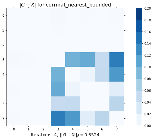
個々の要素の重み付け
近似行列の個々の要素に重み付けできるようにすることは良いでしょうか?
我々の例では、おそらく左上の3×3ブロックの正確な相関関係です。
要素ごとの重み付けは、以下の最小値を求めることを意味します
\[ \Large \|H \circ(G-X) \|_F \]
つまり、個別に \(h_{ij} \times (g_{ij} – x_{ij})\) となります。
しかし、これはより「難しい」問題であり、計算コストも高くなります。
これはnAGルーチン library.correg.corrmat_h_weight で実装されています。
corrmat_h_weightを使用して、要素ごとの重み付けを行った最近接相関行列を計算します
# 重みの行列を設定する
H = np.ones([n, n])
H[:3, :3] = 100
H
array([[100., 100., 100., 1., 1., 1., 1., 1.],
[100., 100., 100., 1., 1., 1., 1., 1.],
[100., 100., 100., 1., 1., 1., 1., 1.],
[ 1., 1., 1., 1., 1., 1., 1., 1.],
[ 1., 1., 1., 1., 1., 1., 1., 1.],
[ 1., 1., 1., 1., 1., 1., 1., 1.],
[ 1., 1., 1., 1., 1., 1., 1., 1.],
[ 1., 1., 1., 1., 1., 1., 1., 1.]])# nAGルーチンを呼び出し、最小固有値を指定する
alpha = 0.001
X, itr, _ = nl_correg.corrmat_h_weight(G, alpha, H, maxit=200)
print("Nearest correlation matrix using element-wise weighting\n{}".format(X))Nearest correlation matrix using element-wise weighting
[[ 1. -0.3251 0.1881 0.5371 0.0255 -0.5893 -0.0625 -0.1929]
[-0.3251 1. 0.2048 0.2249 0.4144 0.2841 0.2914 0.4081]
[ 0.1881 0.2048 1. -0.1462 0.7883 0.2718 -0.6084 0.8804]
[ 0.5371 0.2249 -0.1462 1. 0.2138 -0.0002 0.607 -0.2199]
[ 0.0255 0.4144 0.7883 0.2138 1. 0.6566 -0.2807 0.8756]
[-0.5893 0.2841 0.2718 -0.0002 0.6566 1. 0.0474 0.593 ]
[-0.0625 0.2914 -0.6084 0.607 -0.2807 0.0474 1. -0.4471]
[-0.1929 0.4081 0.8804 -0.2199 0.8756 0.593 -0.4471 1. ]]print("Sorted eigenvalues of X [{0}]".format(
''.join(
['{:.4f} '.format(x) for x in np.sort(np.linalg.eig(X)[0])]
)
))以下はXの固有値を昇順に並べたものです [0.0010-0.0000j 0.0010+0.0000j 0.0375+0.0000j 0.1734+0.0000j 0.6882+0.0000j 1.7106+0.0000j 1.9224+0.0000j 3.4660+0.0000j ]
fig1, ax1 = plt.subplots(figsize=(14, 7))
cax1 = ax1.imshow(abs(X-G), interpolation='none', cmap=plt.cm.Blues, vmin=0,
                  vmax=0.2)
cbar = fig1.colorbar(cax1, ticks = np.linspace(0.0, 0.2, 11, endpoint=True),
                     boundaries=np.linspace(0.0, 0.2, 11, endpoint=True))
cbar.mappable.set_clim([0, 0.2])
ax1.tick_params(axis='both', which='both',
                bottom='off', top='off', left='off', right='off',
                labelbottom='off', labelleft='off')

ax1.set_title(r'$|G-X|$ for corrmat_h_weight', fontsize=16)
plt.xlabel(
    r'Iterations: {0}, $||G-X||_F = {1:.4f}$'.format(itr, np.linalg.norm(X-G)),
    fontsize=14,
)
plt.show()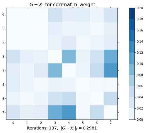
要素のブロックを固定する
おそらく、真の相関の先頭ブロックを固定して、全く変更されないようにしたいと考えています。
nAGルーチンlibrary.correg.corrmat_shrinkingがあります。
このルーチンは先頭ブロックを固定します。このブロックは正定値である必要があります。
Higham、Strabić、Šegoの縮小アルゴリズムを適用します。このアプローチは計算コストが高くありません。
私たちが見つけるのは、Xが真の相関行列となるような最小のαです:
\[ \large X = \alpha \left( \begin{array}{ll}G_{11} & 0 \\ 0 & I \end{array} \right) +(1-\alpha)G, \qquad G = \left( \begin{array}{ll} G_{11} & G_{12} \\ G_{12}^T & G_{22} \end{array} \right) \]
\(G_{11}\)は、固定したい近似相関行列の先頭\(k\)×\(k\)ブロックです。
\(\alpha\)は区間\([0,1]\)にあります。
corrmat_shrinkingを使用して、先頭ブロックを固定した最近接相関行列を計算する
# nAGルーチンを呼び出し、上部3×3ブロックを固定する
k = 3
X, alpha, itr, _, _ = nl_correg.corrmat_shrinking(G, k)
print("Nearest correlation matrix with fixed leading block \n{}".format(X))
Nearest correlation matrix with fixed leading block
[[ 1. -0.325 0.1881 0.4606 0.0051 -0.4887 -0.0579 -0.1271]
[-0.325 1. 0.2048 0.1948 0.3245 0.2183 0.2294 0.3391]
[ 0.1881 0.2048 1. -0.106 0.6124 0.2211 -0.4936 0.7202]
[ 0.4606 0.1948 -0.106 1. 0.2432 0.0101 0.516 -0.2567]
[ 0.0051 0.3245 0.6124 0.2432 1. 0.532 -0.2634 0.7949]
[-0.4887 0.2183 0.2211 0.0101 0.532 1. 0.0393 0.4769]
[-0.0579 0.2294 -0.4936 0.516 -0.2634 0.0393 1. -0.3185]
[-0.1271 0.3391 0.7202 -0.2567 0.7949 0.4769 -0.3185 1. ]]print("Sorted eigenvalues of X [{0}]".format(
''.join(
['{:.4f} '.format(x) for x in np.sort(np.linalg.eig(X)[0])]
)
))
print("Value of alpha returned: {:.4f}".format(alpha))Sorted eigenvalues of X [0.0000 0.1375 0.2744 0.3804 0.7768 1.6263 1.7689 3.0356 ]
Value of alpha returned: 0.2003fig1, ax1 = plt.subplots(figsize=(14, 7))
cax1 = ax1.imshow(abs(X-G), interpolation='none', cmap=plt.cm.Blues, vmin=0,
vmax=0.2)
cbar = fig1.colorbar(cax1, ticks = np.linspace(0.0, 0.2, 11, endpoint=True),
boundaries=np.linspace(0.0, 0.2, 11, endpoint=True))
cbar.mappable.set_clim([0, 0.2])
ax1.tick_params(axis='both', which='both',
bottom='off', top='off', left='off', right='off',
labelbottom='off', labelleft='off')
ax1.set_title(r'$|G-X|$ for corrmat_shrinking', fontsize=16)
plt.xlabel(
r'Iterations: {0}, $||G-X||_F = {1:.4f}$'.format(itr, np.linalg.norm(X-G)),
fontsize=14,
)
plt.show()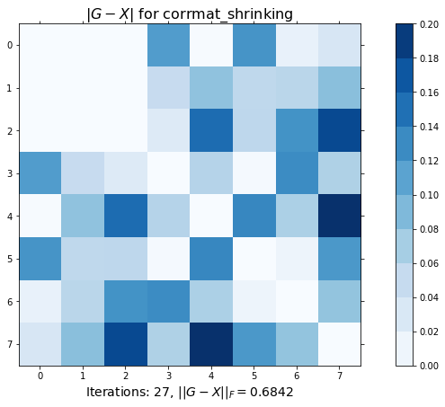
任意の要素の修正
- ルーチン library.correg.corrmat_target は、以下の式で X が真の相関行列となるような最小の α を見つけることで、任意の要素を修正します:
\[ X = \large \alpha T+(1-\alpha)G, \quad T = H \circ G, \quad h_{ij} \in [0,1] \]
H の “1” は G の対応する要素を固定します。
\(0 < h_{ij} < 1\) は G の対応する要素の重みを表します。
\(\alpha\) は再び区間 \([0,1]\) に含まれます。
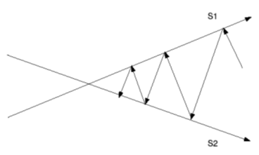
交互射影法
元の問題を解くために最初に提案された方法ですが、非常に遅いです。
アイデアは、以下の2つの集合に交互に射影することです:
- 半正定値行列の集合 (S1)、および
- 対角成分が1の行列の集合 (S2)
これを両方の性質を持つ行列に収束するまで繰り返します。
アンダーソン加速を用いた交互射影法
Higham と Strabić による新しいアプローチは アンダーソン加速 を使用し、この方法を有用なものにします。
特に、フロベニウスノルムにおいて最も近い真の相関行列を見つけながら、要素を固定することができます。
新しい射影は以下のようになります:
- ある最小固有値を持つ(半)正定値行列の集合、および
- 与えられたインデックス \(i\) と \(j\) に対して要素 \(G_{i,j}\) を持つ行列の集合
将来の nAG ライブラリに登場予定です。
nAG ライブラリの Python での使用についての詳細:
https://www.nag.com/nag-library-python