
このページは、nAGライブラリのJupyterノートブックExampleの日本語翻訳版です。オリジナルのノートブックはインタラクティブに操作することができます。
軌道データフィッティング
非線形最小二乗法による軌道データフィッティングの例です。与えられた一連の軌道データ点に対して、軌道経路と固定データ点との間の誤差を最小化する最適な軌道経路を推定することが課題です。
import numpy as np
import math
import matplotlib.pyplot as plt
import matplotlib.patches as pch
from naginterfaces.base import utils
from naginterfaces.library import opt
im = plt.imread("earth.png")
implot = plt.imshow(im)
tx = np.array([441.23, 484.31, 265.15, 98.25, 180.66, 439.13, 596.54])
ty = np.array([333.92, 563.46, 577.40, 379.23, 148.62, 100.28, 285.99])
cc = np.array([355.00, 347.00])
tr = (tx-cc[0])**2 + (ty-cc[1])**2
plt.plot(tx,ty,'y+')
plt.axis('off')
plt.savefig('dat_orbit.png', bbox_inches='tight', dpi=150)
plt.show()
画像クレジット: 地球の画像はEUMETSAT、著作権2020から取得しました。
前の画像は、最適な軌道 r
を推定する必要がある軌道測定値を示しています。
解決すべき単純な単変量問題は次のとおりです:
![LaTeX equation: min f(x) = sum i=1 to nres of (tr[i]^2 - r2)2](ltx_optprb.png)
ここで tr[i] は、座標ペア (tx[i], ty[i])
で与えられる測定点 i
の二乗ノルムを含んでいます。惑星の中心の座標はベクトル cc
で提供されていることに注意してください。
# 問題データ
# 観測数
nres = len(tx)
# 観測値
# コールバック関数に渡されるデータ構造を定義する
data = {'tr': tr}
# フィッティングするパラメータの数
nvar = 1
# 最小二乗関数を定義し、一次導関数を追加します。
def lsqfun(x, nres, inform, data):
"""
Objective function call back passed to the least squares solver.
Return the difference between the current estimated radius squared, r^2=x^2 and
the squared norm of the data point stored in tr[i] for i = 1 to nres:
rx[i] = r^2 - tr[i], i = 1, ..., nres.
"""
rx = x**2 - data['tr']
return rx, inform
def lsqgrd(x, nres, rdx, inform, data):
"""
Computes the Jacobian of the least square residuals.
Simply return rdx[i] = 2r, i = 1, ..., nres.
"""
rdx[:] = 2.0*np.ones(nres)*x[:]
return inform# モデルハンドルを初期化する
handle = opt.handle_init(nvar)
# 密な非線形最小二乗目的関数を定義する
opt.handle_set_nlnls(handle, nres)# パラメータ空間を制限する (0 <= x)
opt.handle_set_simplebounds(handle, np.zeros(nvar), 1000.0*np.ones(nvar))# ソルバーの出力を制御するためのオプションパラメータを設定する
for option in [
'Print Options = NO',
'Print Level = 1',
'Print Solution = X',
'Bxnl Iteration Limit = 100'
]:
opt.handle_opt_set(handle, option)
# 省略された反復出力のために明示的なI/Oマネージャーを使用する:
iom = utils.FileObjManager(locus_in_output=False)# 初期推定値(開始点)をゼロから離れた値に定義します。ゼロは問題を引き起こす可能性があります。
x = np.ones(nvar)ソルバーを呼び出す
# Call the solver
slv = opt.handle_solve_bxnl(handle, lsqfun, lsqgrd, x, nres, data=data, io_manager=iom)
E04GG, Nonlinear least squares method for bound-constrained problems
Status: converged, an optimal solution was found
Value of the objective 1.45373E+09
Norm of projected gradient 2.23690E-01
Norm of scaled projected gradient 4.14848E-06
Norm of step 3.75533E-06
Primal variables:
idx Lower bound Value Upper bound
1 0.00000E+00 2.38765E+02 1.00000E+03# 最適なパラメータ値
rstar = slv.x
print('Optimal Orbit Height: %3.2f' % rstar)Optimal Orbit Height: 238.76figure, axes = plt.figure(), plt.gca()
implot = plt.imshow(im)
orbit = plt.Circle(cc, radius=rstar, color='w', fill=False)
axes.add_patch(orbit)
plt.plot(tx, ty, 'y+')
plt.axis('off')
plt.savefig('est_orbit.png', bbox_inches='tight', dpi=150)
plt.show()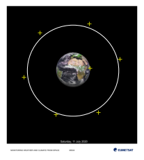
専門家の知識により、各測定の信頼性に関する洞察が得られ、この衛星構成では、運用軌道高度は約250 ±6単位であるべきだとします。前の画像は、各測定(データポイント)が同じ量だけ寄与し、最適な軌道高度が238.76単位となるフィットを示しています。このフィットは、専門家のアドバイスを満たしていないという意味で、かなり不十分です。明らかにデータポイント0(地球表面に最も近い黄色の十字)は信頼性が低いです。フィッティングを行う際には、この信頼性の低さを考慮に入れる必要があります。このため、各残差に対する重みが導入されます(重みは変動性の逆数に比例するように設定されるべきです)。この例では、各データ測定の精度が提供されていると仮定します。
この新しい情報を用いて、重み付き非線形最小二乗法を使用して問題を再度解きます。
# 各残差に重みを追加
weights = np.array([0.10, 0.98, 1.01, 1.00, 0.92, 0.97, 1.02])
weights /= weights.sum()

# 測定値(重み)の信頼性を定義する
opt.handle_set_get_real(handle, 'rw', rarr=weights)

# ソルバーに重みを使用することを指示する
for option in [
        'Bxnl Use weights = Yes',
]:
    opt.handle_opt_set(handle, option)

# もう一度解く
slv = opt.handle_solve_bxnl(handle, lsqfun, lsqgrd, x, nres, data=data, io_manager=iom) # monit=monit,

# 目的と解決策
rstar = slv.x
print('Optimal Orbit Height: %3.2f' % rstar)
E04GG, Nonlinear least squares method for bound-constrained problems
Status: converged, an optimal solution was found
Value of the objective 1.25035E+06
Norm of projected gradient 6.26959E-03
Norm of scaled projected gradient 3.96468E-06
Norm of step 8.72328E-03
Primal variables:
idx Lower bound Value Upper bound
1 0.00000E+00 2.54896E+02 1.00000E+03
Optimal Orbit Height: 254.90figure, axes = plt.figure(), plt.gca()
implot = plt.imshow(im)
orbit = plt.Circle(cc, radius=rstar, color='w', fill=False)
axes.add_patch(orbit)
plt.plot(tx, ty,'y+')
plt.axis('off')
plt.savefig('estw_orbit.png', bbox_inches='tight', dpi=150)
plt.show()
print('Optimal Orbit Height: %3.2f (should be between 244 and 256)' % rstar)
Optimal Orbit Height: 254.90 (should be between 244 and 256)この重み付けモデルでは、提供された軌道解は専門家のアドバイスと一致しています。